TikZ
There is a variety of different toolsets for creating graphical objects in a TeX document. The most well known and probably most widely used of these toolsets is TikZ, which is a recursive acronym for “TikZ ist kein Zeichenprogramm” (German for TikZ is not a drawing programme). From the name of the toolset you can see that generating a figure in TikZ will not work through drawing the figure like you might be familiar with doing in Paint or similar drawing programmes. To create a figure using TikZ you will need to code it by using specific TeX commands. We will take a look at the basics of TikZ here.
Three useful references and sources of inspiration for creating TikZ figure are:
- The Wikibooks entry on TikZ: https://en.wikibooks.org/wiki/LaTeX/PGF/TikZ.
- The CTAN entry on TikZ with the official handbook and other documentation: https://www.ctan.org/pkg/pgf.
- The TeXample TikZ database full of examples and inspiration: https://texample.net/tikz/.
Building blocks of TikZ
To create a figure in TikZ you will first need to load the correct package in your TeX file, i.e. use \usepackage{tikz} in the preamble. There is a wide range of options and special TikZ libraries which can also be used and would need to be loaded specifically, but we will not need these in this beginner course. You can look at the available options and try them out yourself using the three references given above.
A TikZ figure is usually placed in a \begin{figure} LaTeX environment, as you would do with other figures. This is useful because it will allow you to give the figure a number and caption, so that you will be able to reference it easily. Within your figure environment you can start a TikZ figure by writing the code \begin{tikzpicture}, after which you can start typesetting your figure. As usual you close the environment with the code \end{tikzpicture}.
Unlike you are used to when typesetting text and mathematics in LaTeX, you will need one character which does not correspond directly to something you can see in your document. Every line of TikZ code must be closed with a semicolon.
Let us get started by typesetting a graph, step by step, in TikZ. At the end of this lesson we will be able to typeset the following figure.
Drawing lines
A graph consists of several points and lines. We start the drawing of a graph by defining the coordinates of the points. In TikZ this can be done in two different ways. A cartesian coordinate is given by two numbers (an x- and a y-coordinate) separated by a comma, and surrounded by round brackets, so (-2,0) or (1.5,1.5). In TikZ coordinates can also be given in polar form. This also works by giving two numbers inside round brackets (the angle in degrees, and the length), this time separated by a colon, so (180:2) or (45:2.1) for (approximately) the same two coordinates. Note: when no unit of measurement is given the default is centimeters, coordinates can also be given as (1cm, 2pt) for example.
We can now draw direct straight lines between these coordinates using the \draw command.
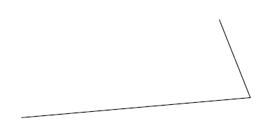
\begin{tikzpicture}
  \draw (-1,0) -- (3,10pt) -- (35:3);
\end{tikzpicture}
The result of this code is the following image.
Apart from the drawing of direct straight lines, we can also define other types of lines, and these lines can be given colour, line thickness, or pattern. For example, use -| or |- in stead of -- to draw lines that go horizontal first and then vertical, or the other way around.
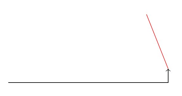
The style of the lines can be changed by giving options to the \draw command. This is done by putting these options in square brackets behind the command. In the following example we draw an arrow in stead of a line, and give another line a colour.
\begin{tikzpicture}
  \draw[->] (-1,0) -| (3,10pt);
  \draw[red] (3,10pt) -- (35:3);
\end{tikzpicture}
The result of this code is the following image.
Use the TikZ sources to see which types of options are possible.
We can not only draw straight lines, but also curved lines. This can be done in several different ways. In the following example we present three options.
\begin{tikzpicture}
  \draw (-1,0) to (5,1);
  \draw[green] (-1,0) to[out=90,in=135] (5,1);
  \draw[cyan] (-1,0) .. controls (0,-2) .. (5,1);
\end{tikzpicture}
The result of this code is the following image.
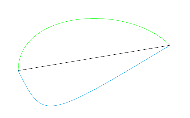
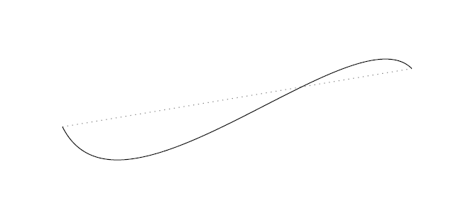
The first thing that you might notice is the use of to in stead of -- to connect the coordinates together. This command works in exactly the same way, but when using to we can add options to the connecting command. For the green line we give two options, firstly the angle (in degrees) at which the line departs from the first coordinate, and secondly the angle at which the line arrives at the second coordinate. The blue line is a so called Bézier curve, this is a line defined by its begin and end points together with a number of support points (in this case one) that in effect draw the line toward themselves. In TikZ these types of lines can be defined with either one or two support points. In the example below we give the code to draw a Bézier curve with two support points.
\begin{tikzpicture}
  \draw[dotted,gray] (-1,0) -- (5,1);
  \draw (-1,0) .. controls (0,-2) and (4,2) .. (5,1);
\end{tikzpicture}
The result of this code is the following image.
Nodes
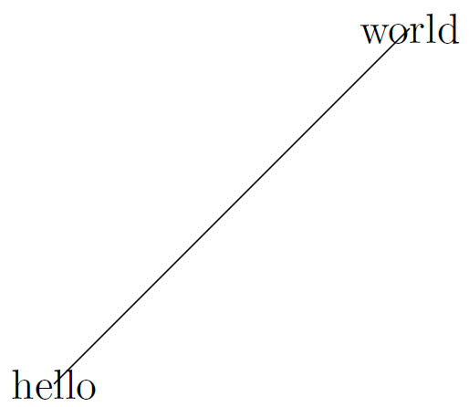
The next step on the way to typesetting a graph are the labels, the bits of text and numbers that are contained in the figure. To write text in a TikZ figure we need an object called a node. The simplest example of a node is some text which is placed on a given coordinate, but a node can also be a bit of text surrounded by a circle, rectangle, or other simple shape. A node does not necessarily need to contain text, but for most cases text is the purpose of the node. A node can be defined while drawing a path, which works as follows:
\begin{tikzpicture}[scale=3]
  \draw (0,0) node {hello} -- (1,1) node {world};
\end{tikzpicture}
The result of this code is the following image.
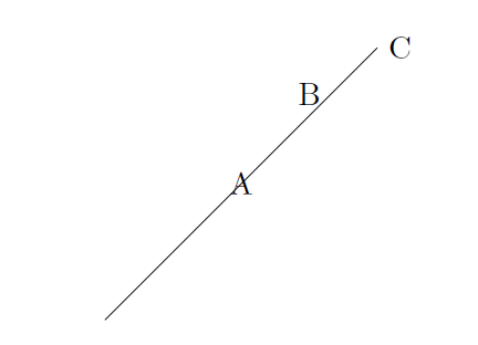
The option [scale=3] at the beginning of the figure increases the scale of the figure with a factor 3. The command node can also be given options, for example to place a node in the middle of a line, at the end of a line, etc.
\begin{tikzpicture}[scale=3]
  \draw (0,0) -- (1,1) node[midway]{A} node[pos=0.75,above]{B} node[right]{C};
\end{tikzpicture}
The result of this code is the following image.
Please note: when using the command to rather than --, the location of the node command changes slightly. This following example code generates the same image as given above.
\begin{tikzpicture}[scale=3]
  \draw (0,0) to node[midway]{A} node[pos=0.75, above]{B} (1,1) node[right]{C};
\end{tikzpicture}
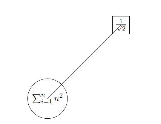
Nodes can also be given mathematical formulae, and as has been said they can be bordered by a simple shape.
\begin{tikzpicture}[scale=3]
  \draw (0,0) node[circle, draw]{$\sum_{i=1}^{n}n^2$} -- (1,1)
  node[rectangle,draw]{$\frac{1}{\sqrt{2}}$};
\end{tikzpicture}
The result of this code is the following image.
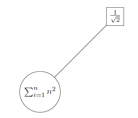
As you might have spotted, the line connecting the nodes still starts and ends exactly in the defined coordinates, which is not very pretty. This can be solved by predefining the nodes, and giving them a label, so that we can draw the line from node to node.
\begin{tikzpicture}[scale=3]
  % define nodes
  \node[circle,draw] (label1) at (0,0) {$\sum_{i=1}^{n}n^2$};
  \node[rectangle,draw] (label2) at (1,1) {$\frac{1}{\sqrt{2}}$};

  % draw the line
  \draw (label1) -- (label2);
\end{tikzpicture}
The result of this code is the following image.
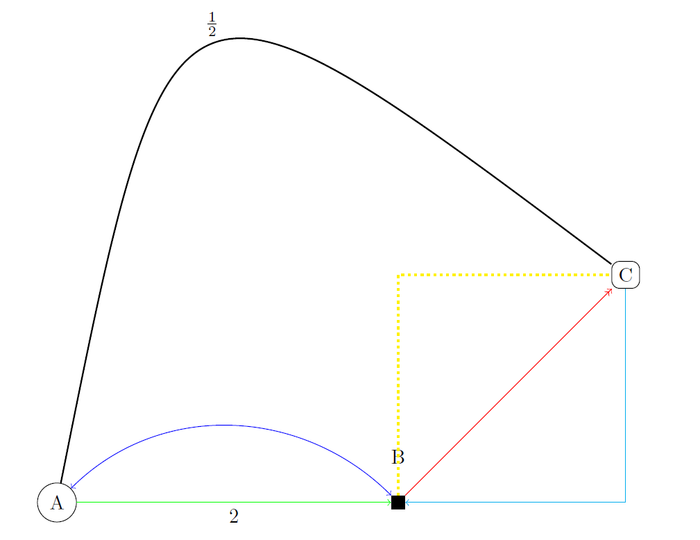
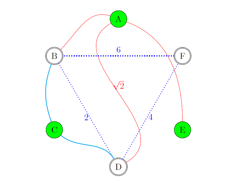
We have now seen sufficient examples to understand how a graph can be typeset in TikZ. The next bit of code is the code used to generate the graph seen at the beginning of this lesson.
\begin{tikzpicture}[scale=2]
  % Define the nodes
  \node[circle, draw] at (0,0) (a) {A};
  \node[rectangle, fill] at (3,0) (b) {};
  \node at (3,0.4) (blabel) {B};
  \node[rectangle,rounded corners, draw] at (5,2) (c) {C};

  % Draw the paths
  \draw[->, green] (a) -- (b) node[midway, below,black]{2};
  \draw[<->, blue] (a) to[out=45, in=135] (b);
  \draw[->>,red] (b)--(c);
  \draw[yellow,dotted,very thick] (b) |- (c);
  \draw[<-,cyan] (b) -| (c);
  \draw[thick,black] (a).. controls (1,5) .. (c) node[midway, above]{$\frac{1}{2}$};
\end{tikzpicture}
Exercise 1
It is time to try some typesetting yourself. Open your favourite TeX editor and try to typset graph below this exercise: The graph does not need to look exactly the same as the image, the point is that you are able to typeset a graph with similar properties. Hint: It might help to define the nodes in a circle using polar coordinates. You may copy this code for the document structure, so that you only need to focus on TikZ.
\documentclass[border=1cm]{standalone}
\usepackage{tikz}
\begin{document}
\end{document}
Plotting curves
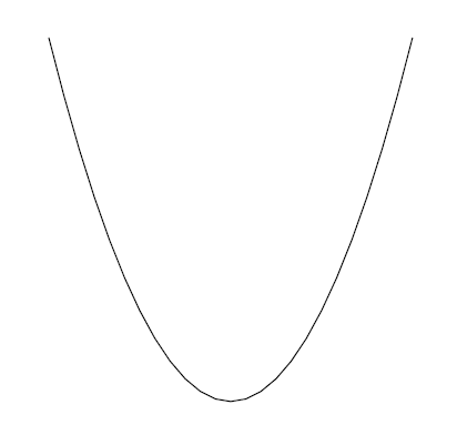
It is not only possible to draw lines between coordinates in TikZ. There is also a built in way to plot curves of a large range of different functions. For example the function $y = x^2$ on the interval $[-2, 2]$.
\begin{tikzpicture}
  \draw [domain=-2:2] plot (\x, {pow(\x,2});
\end{tikzpicture}
The result of this code is the following image.
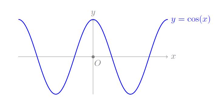
By using what you have learned in the previous sections, you can add axes and labels to this curve. For example:
\begin{tikzpicture}[scale=1.5]
  % Draw the x and y axis, label the axes and the origin
  \draw[gray, ->] (-2,0) -- (2,0) node[right]{$x$} node[pos=0.53, below]{$O$};
  \draw[gray, ->] (0,-1) -- (0,1) node[above]{$y$};
  \draw[fill,gray] (0,0) circle [radius=1pt];

  % Plot the curve
  \draw[blue, thick] [domain=-2:2, samples=150] plot (\x, {cos(pi*\x r)})
  node[right]{$y = \cos(x)$};
  % Note: the r in the argument of the cosine signifies that we enter \x in radians
\end{tikzpicture}
The result of this code is the following image.
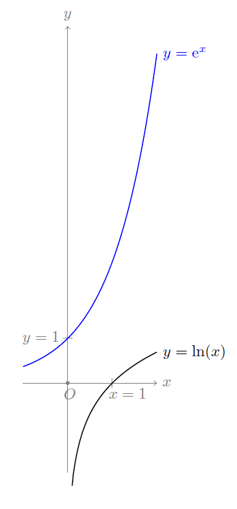
Exercise 2
Try to typset the plot following this exercise. You may copy this code for the document structure, so that you only need to focus on TikZ.
\documentclass[border=1cm]{standalone}
\usepackage{tikz}
\begin{document}
...
\end{document}
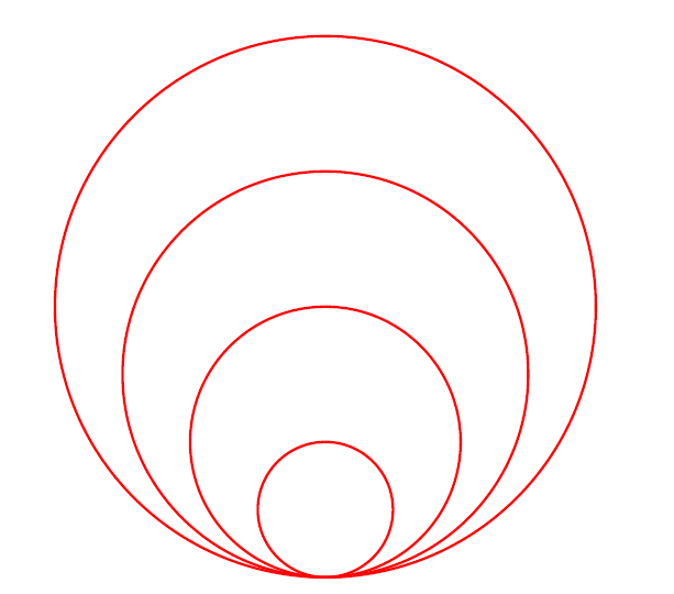
Working with loops
In TikZ it is also possible to make use of for loops, using \foreach ... in .... In this way, a fairly complicated image can be typeset very quickly.
\begin{tikzpicture}[scale=0.75]
  \foreach \x in {0,1,2,3}
  \draw[red,thick] (0,\x) circle [radius=\x+1];
\end{tikzpicture}
The result of this code is the following image.
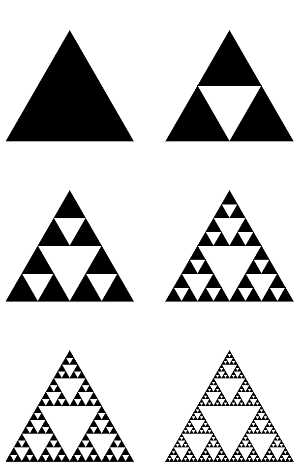
This idea is very useful for drawing iterative figures like Sierpiński’s triangle, although that does require a special TikZ library with which a recursive function can be defined. The following code gives the first six iterations of Sierpiński’s triangle, drawn in TikZ. The code also contains some things in the preamble (before \begin{document}), so we give the full LaTeX code for a pdf with only this figure in it.
\documentclass[border=1cm]{standalone}

\usepackage{tikz}
\usetikzlibrary{math}

% Define a equilateral triangle with lower left corner at coordinate #1 and
% with length of the sides #2
\newcommand\Triangle[2]{
  \draw #1 coordinate(a)  -- ++(0:#2) coordinate(b) ;
  \draw (a) -- ++(60:#2) coordinate(c);
  \fill (a) -- (b) -- (c) -- cycle;
}

\begin{document}
\begin{tikzpicture}
  \tikzmath{
    % Define the recursive function sierpinski
    function sierpinski(\x, \y, \s, \d) {
      if (\d == 0) then {
        % Draw a triangle lower left corner at (\x, \y), length \s
        { \Triangle{(\x,\y)}{\s}; };
			} else {
        % Rescale the length of the sides and choose correct coords
	% for the next triangles
        \u1 = 0.25*\s;
        \u2 = \u1*sqrt(3);
        \u3 = 0.5*\s;
        sierpinski(\x,\y,\u3,\d-1);
        sierpinski(\x+\u3,\y,\u3,\d-1);
        sierpinski(\x+\u1,\y+\u2,\u3,\d-1);
      };
    };
    % Let the length of the sides of the base triangle be 4, and generate 6 figures
    \S = 4;
    for \d in {0,...,5}{
      % To situate all plots nicely under and next to each other, define the coords
      % of the lower left corners preemptively
      \x = (\S+1)*mod(\d,2);
      \y = int(\d/2) * (\S+1);
      sierpinski(\x,-\y,\S,\d);
      };
  }
\end{tikzpicture}
\end{document}
The result of this code is the following image.
Exercise 3 (bonus)
Copy the code for the Sierpiński triangles given above, and try to adapt it so that you can generate a figure displaying several iterations of the Sierpiński carpet (see also Wikipedia: https://en.wikipedia.org/wiki/Sierpi%C5%84ski_carpet).